
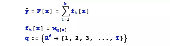
Xgboost is an integrated learning algorithm, which belongs to the category of boosting algorithms in the 3 commonly used integration methods (bagging, boosting, stacking). It is an additive model, and the base model is usually chosen as a tree model, but other types of models such as logistic regression can also be chosen.
1. xgboost and GBDT
Xgboost belongs to the category of gradient boosted tree (GBDT) models. The basic idea of GBDT is to let the new base model (GBDT takes CART categorical regression tree as the base model) to fit the deviation of the previous model, so as to continuously reduce the deviation of the additive model.
Compared with the classical GBDT, xgboost has made some improvements, resulting in significant improvements in effectiveness and performance (highlighting a common interview test).
-
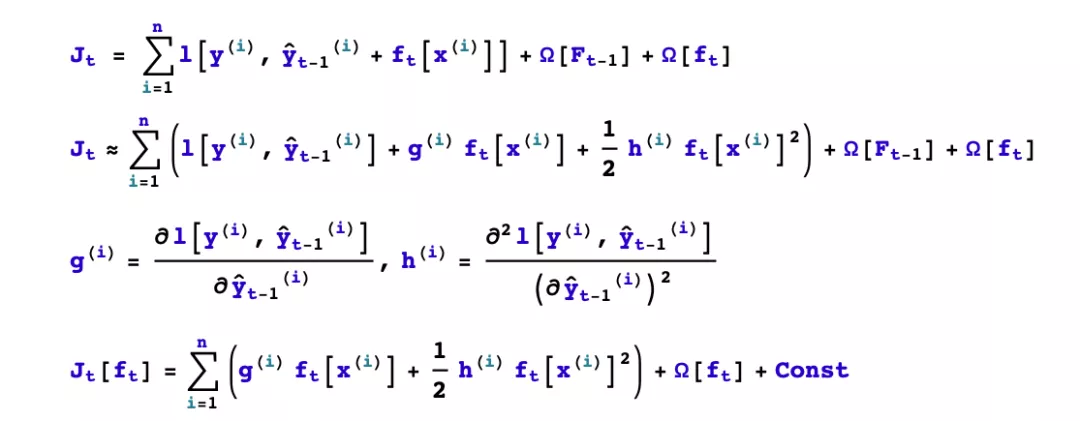
GBDT expands the objective function Taylor to the first order, while xgboost expands the objective function Taylor to the second order. More information about the objective function is retained, which helps to improve the effect.
-
GBDT is finding a new fit label for the new base model (negative gradient of the previous additive model), while xgboost is finding a new objective function for the new base model (second-order Taylor expansion of the objective function about the new base model).
-
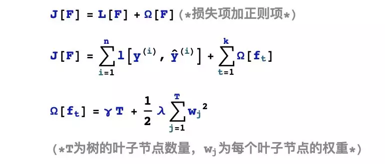
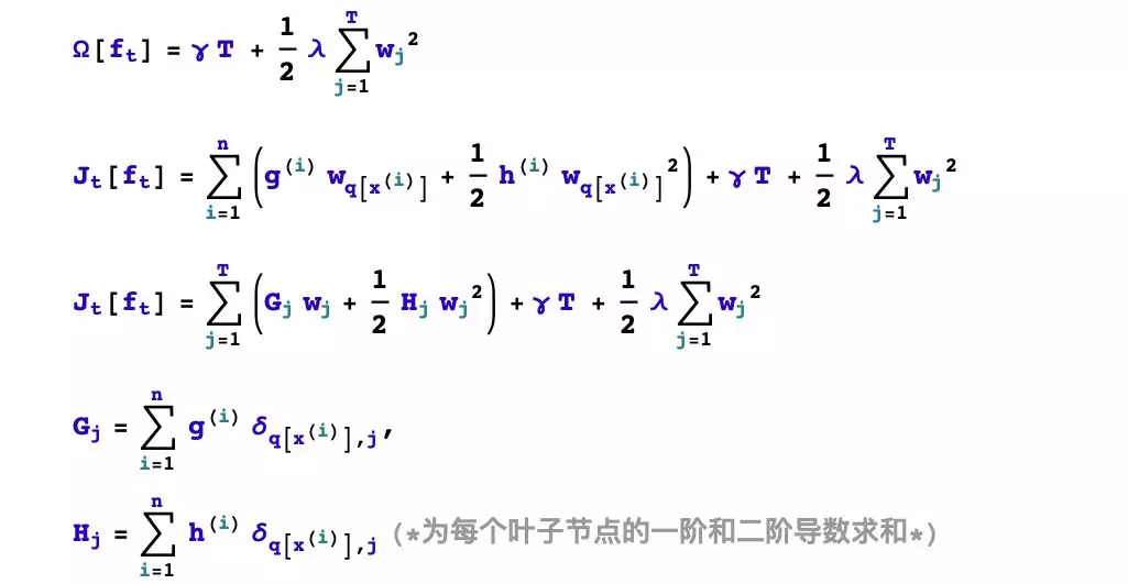
xgboost adds and L2 regularization term for the leaf weights, thus facilitating the model to obtain a lower variance.
-
xgboost adds a strategy to automatically handle missing value features. By dividing the samples with missing values into left subtree or right subtree respectively and comparing the advantages and disadvantages of the objective functions under the two schemes, the samples with missing values can be divided automatically without the need of filling preprocessing the missing features.
In addition, xgboost also supports candidate quantile cuts, feature parallelism, etc., which can improve performance.
2. xgboost Basic Principle
The following is a general introduction to the principle of xgboost from three perspectives: assumption space, objective function, and optimization algorithm.
1. Hypothesis space
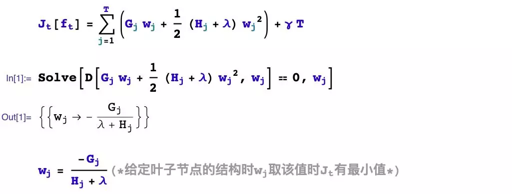
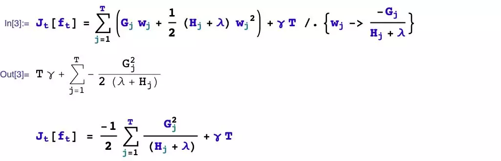
2. Objective function
3. Optimization algorithm
The basic idea: greedy method, learning tree by tree, each tree fits the deviation of the previous model.
Third, the first t trees to learn what? To finish building the xgboost model, we need to determine some of the following things.
-
how to boost? If the additive model composed of the previous t-1 trees has been obtained, how to determine the learning goal of the tth tree?
-
How to generate the tree? If the learning goal of the tth tree is known, how to learn this tree? Specifically, does it involve splitting or not? Which feature is selected for splitting? What splitting point is chosen? How to take the value of the split leaf nodes?
We first consider the problem of how to boost, and then solve the problem of how to take the values of the split leaf nodes.
4. How to generate the tth tree?
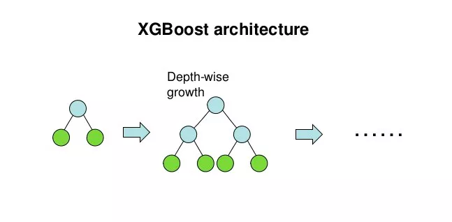
xgboost uses a binary tree, and at the beginning, all the samples are on one leaf node. Then the leaf nodes are continuously bifurcated to gradually generate a tree.
xgboost uses a levelwise generation strategy, i.e., it tries to split all the leaf nodes at the same level at a time.
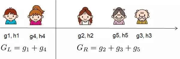
The process of splitting leaf nodes to generate a tree has several basic questions: should we split? Which feature to choose for splitting? At what point of the feature to split? and what values are taken on the new leaves after the split?
The problem of taking values of leaf nodes has been solved earlier. Let’s focus on a few remaining questions.
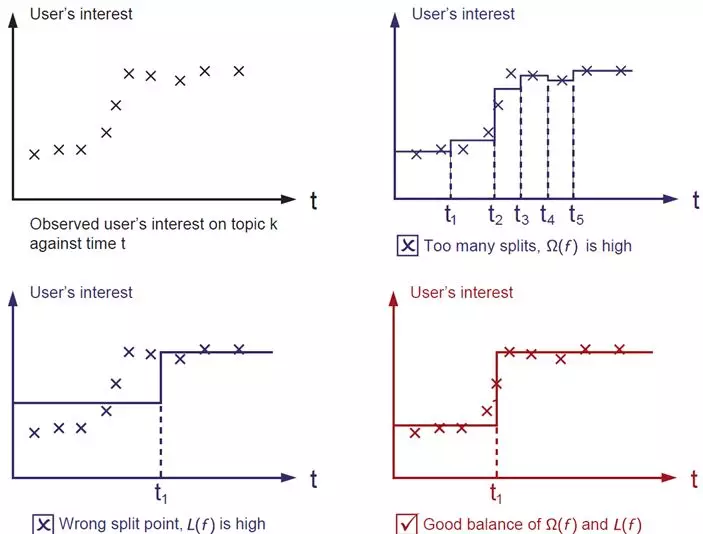
- Should splitting be performed?
Depending on the pruning strategy of the tree, this problem is handled in two different ways. If it is a prepruning strategy, then splitting will be done only if there is some way of splitting that makes the objective function drop after splitting.
However, if it is a post-pruning strategy, the splitting will be done unconditionally, and then after the tree generation is completed, the branches of the tree will be checked from top to bottom to see if they contribute positively to the decline of the objective function and thus pruned.
xgboost uses a prepruning strategy and splits only if the gain after splitting is greater than 0.

- What features are selected for splitting?
xgboost uses feature parallelism to select the features to be split, i.e., it uses multiple threads to try to use each feature as a splitting feature, find the optimal splitting point for each feature, calculate the gain generated after splitting them, and select the feature with the largest gain as the splitting feature.
- What splitting point is selected?
There are two methods for xgboost to select the splitting point of a feature, one is the global scan method and the other is the candidate splitting point method.
The global scan method arranges all the values of the feature in the sample from smallest to largest, and tries all the possible splitting locations to find the one with the greatest gain, whose computational complexity is proportional to the number of different values of the sample feature on the leaf node.
In contrast, the candidate split point method is an approximate algorithm that selects only a constant number (e.g., 256) of candidate split positions, and then finds the best one from the candidate split positions.
5. Example of xgboost usage
You can use pip to install xgboost
pip install xgboost
The following is an example of using xgboost, you can refer to modify the use.
import numpy as np
import pandas as pd
import xgboost as xgb
import datetime
from sklearn import datasets
from sklearn.model_selection import train_test_split
from sklearn.metrics import accuracy_score

def printlog(info):
    nowtime = datetime.datetime.now().strftime('%Y-%m-%d %H:%M:%S')
    print("\n "+"=========="*8 + "%s"%nowtime)
    print(info+'... \n\n')


# ================================================================================
# I. Reading data
# ================================================================================
printlog("step1: reading data...")

# read dftrain,dftest
breast = datasets.load_breast_cancer()
df = pd.DataFrame(breast.data,columns = [x.replace(' ','_') for x in breast.feature_names])
df['label'] = breast.target
dftrain,dftest = train_test_split(df)

xgb_train = xgb.DMatrix(dftrain.drop("label",axis = 1),dftrain[["label"]])
xgb_valid = xgb.DMatrix(dftest.drop("label",axis = 1),dftest[["label"]])

# ================================================================================
# Two, set the parameters
# ================================================================================
printlog("step2: setting parameters...")

num_boost_rounds = 100
early_stopping_rounds = 20

# Configure xgboost model parameters
params_dict = dict()

# booster parameters
params_dict['learning_rate'] = 0.05 # Learning rate, usually smaller is better.
params_dict['objective'] = 'binary:logistic'

# tree parameters
params_dict['max_depth'] = 3 # depth of the tree, usually between [3,10]
params_dict['min_child_weight'] = 30 # minimum leaf node sample weight sum, the larger the model the more conservative.
params_dict['gamma']= 0 # Minimum drop value of loss function required for node splitting, the larger the model the more conservative.
params_dict['subsample']= 0.8 # horizontal sampling, sample sampling ratio, usually between [0.5, 1].
params_dict['colsample_bytree'] = 1.0 # longitudinal sampling, feature sampling ratio, usually between [0.5, 1
params_dict['tree_method'] = 'hist' # strategy for constructing the tree, can be auto, exact, approx, hist

# regulazation parameters
# Omega(f) = gamma*T + reg_alpha* sum(abs(wj)) + reg_lambda* sum(wj**2)
params_dict['reg_alpha'] = 0.0 #L1 weight coefficient of the regularization term, the larger the model the more conservative it is, usually takes a value between [0,1].
params_dict['reg_lambda'] = 1.0 #L2 The weight coefficient of the regularization term, the larger the model the more conservative it is, usually takes a value between [1,100].

# Other parameters
params_dict['eval_metric'] = 'auc'
params_dict['silent'] = 1
params_dict['nthread'] = 2
params_dict['scale_pos_weight'] = 1 # Setting to positive value for unbalanced samples will make the algorithm converge faster.
params_dict['seed'] = 0


# ================================================================================
# Third, train the model
# ================================================================================
printlog("step3: training model...")


result = {}
watchlist = [(xgb_train, 'train'),(xgb_valid, 'valid')]

bst = xgb.train(params = params_dict, dtrain = xgb_train,
                num_boost_round = num_boost_round,
                verbose_eval= 1,
                evals = watchlist,
                early_stopping_rounds = early_stopping_rounds,
                evals_result = result)

# ================================================================================
# IV, Evaluation Model
# ================================================================================
printlog("step4: evaluating model ...")


y_pred_train = bst.predict(xgb_train, ntree_limit=bst.best_iteration)
y_pred_test = bst.predict(xgb_valid, ntree_limit=bst.best_iteration)

print('train accuracy: {:.5} '.format(accuracy_score(dftrain['label'], y_pred_train>0.5)))
print('valid accuracy: {:.5} \n'.format(accuracy_score(dftest['label'], y_pred_test>0.5)))

%matplotlib inline
%config InlineBackend.figure_format = 'svg'

dfresult = pd.DataFrame({(dataset+'_'+feval): result[dataset][feval]
               for dataset in ["train", "valid"] for feval in ['auc']})

dfresult.index = range(1,len(dfresult)+1)
ax = dfresult.plot(kind='line',figsize=(8,6),fontsize = 12,grid = True)
ax.set_title("Metric During Training",fontsize = 12)
ax.set_xlabel("Iterations",fontsize = 12)
ax.set_ylabel("auc",fontsize = 12)


ax = xgb.plot_importance(bst,importance_type = "gain",xlabel='Feature Gain')
ax.set_xlabel("Feature Gain",fontsize = 12)
ax.set_ylabel("Features",fontsize = 12)
fig = ax.get_figure()
fig.set_figwidth(8)
fig.set_figheight(6)

# ================================================================================
# v. Save the model
# ================================================================================
printlog("step5: saving model ...")
model_dir = "data/bst.model"
print("model_dir: %s"%model_dir)
bst.save_model(model_dir)
bst_loaded = xgb.Booster(model_file=model_dir)

printlog("task end...")